Typical approach to asset failure

Depending on the nature of assets failure can be expressed either as the number of failures in a year or the probability of failure in a year.

In the case of pipeline where assets are identified in sections researches had indicated that the cumulative number of failures in an asset is distributed as a Poisson variable with mean.

Mean No. of failures = lTtß

Where
l: total length of pipeline, (m)
t: age of asset in years
T: a constant which depends on failure numbers and the environmental conditions
ß: a characteristic of the asset which depends on the failure time histories, can be assumed to be the same for similar assets.

One problem faced by many water authorities involves the prediction of failures as compared with the actual failures that may occur. As pipelines age and their condition deteriorates the number of failures varies significantly due to many variables such as:

• Original construction quality
• Variable decay rates
• Material weaknesses and rate of decay
• Environmental factors such as ground conditions etc.
• Operational factors such as water hammer and other stresses
• External loadings and stresses
• Ground movement.

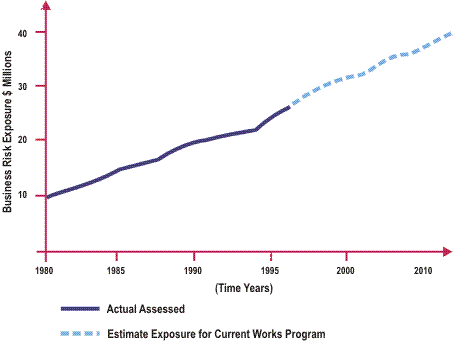
In general the numbers of failures will vary significantly from year to year and as such we often find it difficult to determine the accurate long term trends for these failures.

This is shown below:

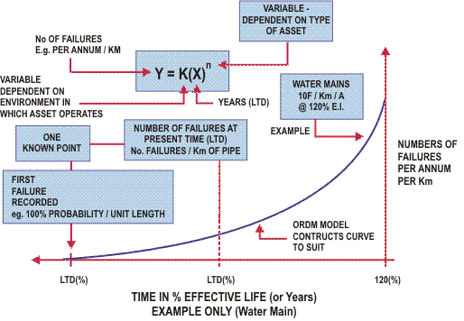
The overall trends of failures, disregarding those failures that are not associated with the age of the pipeline equates to the formula shown in the following diagram.

The basis of typical approach to this study has been to:

• Assess the condition of the pipeline, looking at the various distress failure modes and to score these modes in such a way as to allow the rating of condition of individual sections of the pipeline
• Relate these condition scores to the performance of the pipeline and to determine approximate effective lives for the parent assets
• Develop decay curves that can relate the predicted condition to a predicted performance
• Assess the cost of this predicted performance.

The condition decay curves and predictive models are then used and relate these to the current probability of failure on a time scale for individual assets which are discrete (e.g. pumps).

Instead of working with the cumulative numbers of failure for a group of assets such as for 1000 meter sections of water main the approach is to develop a generic approach for a single asset or groups of assets and to represent the failure with a probability curve of the exponential form.

y = k x n

where
y: probability of failure
k: a constant which depends on the environmental conditions
x: the age of the asset in years
n: a constant which depends on the asset type.

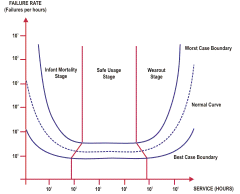
Implicit in the exponential expression for the probability of failure is the assumption that the failure rate follow the increasing trend over the asset's entire operating life. But in the case of dynamic assets involving many individual functional parts the failure rates of individual components are not constant over the assets entire useful life.

Research based on life time testing on production costs of different kinds of parts suggested three successive stages of failure phenomena represented by a bath-tub curve, as shown in the following figure.

A family of failure curves can be developed for each asset or group of assets based on the environmental factors such as the ground conditions, the stresses to which the assets are being subjected to, the maintenance practice in the past.

The approach is to determine the probability of when the first failure will occur, i.e. the time you are 100% confident that an asset would have failed.

In this approach the probability of 100% confidence that an asset would have failed at a given time is assigned a probability of failure of 1.0 at the time of actual failure. The probabilities of failure during the interim period can be determined based on four different failure mode scenarios which are to a large extent influenced by the operating environment:

• Conservative Failure Mode
• Early Failure Mode
• Most Likely Failure Mode
• Late Failure Mode.

In the conservative failure mode, the condition of the asset is assumed to deteriorate consistently and the probability of failure increases linearly from zero when the asset is new to a value of 1.0 when the asset reaches the end of its effective life. This is typically a theoretical failure mode without taking into consideration the actual condition of the asset.

In the most likely failure mode scenario the asset is assumed to exhibit the normal decay profile when operating under the accepted appropriate asset management practices. As typical of passive assets with slow decay in the early stages of their lives the probabilities of failure during the early stage of the asset life are expected to be low but as the asset ages the probabilities of failure begin to increase rapidly. It is envisaged that this type of failure mode will encompass the majority of assets.

Some assets may exhibit an early failure mode because of the less than optimal maintenance and operations strategies or because of the inherent nature of the assets which require "run-in" period with early glitches. However, once the early failure aberrations had been rectified, the assets would then normally follow the probability decay of the average assets.

Under the late failure mode scenario the assets exhibit lower than average probability of failure during the early stages of their lives. These are assets which are usually underutilized during the early part of their lives or assets which have received more than the required amount of maintenance. The assets might have been neglected at the later stages of their lives or the operating environment in which they exist might have become less favorable.