Optimized Renewal Decision Making

The number of failures or the probability of failure will impact the maintenance / repair cost required on the asset.

Using this data, we are then able to predict the future costs likely to be incurred and these are shown in the following figure.

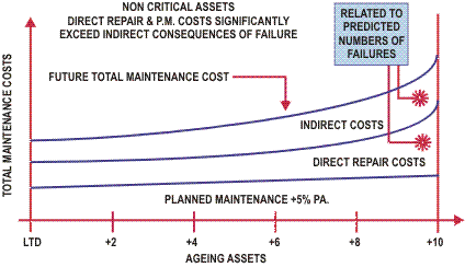
Different treatment options are then assessed against this predicted cost and the potential savings are recognized.

By completing a cash flow of the various options the most cost effective option can be identified as shown in the following figure.

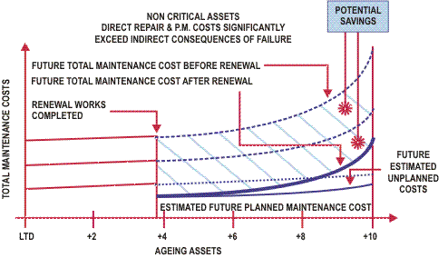
The potential savings for each option will vary with time and it is desirable to identify the most cost effective point for the renewal to be completed.

This is shown in the following figure.

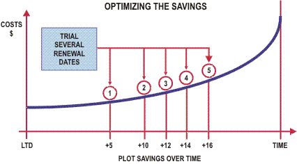
By completing this type of analysis, we can then identify the point at which the greatest potential savings or highest NPV is likely to occur and determine that as the point for which renewals should take place.

This is shown by the following example.

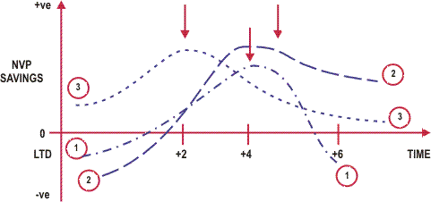
As can be seen this detailed analysis requires significant inputs through both the number of sensitivity assessments and the various timing of the options.

Process flowchart for developing "Appropriate Probability Of" failure curves

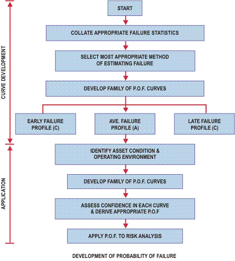
A process flow chart for developing appropriate probability of failure curves is shown below:

Collate "Condition/Failure Statistics" in relation to asset effective lives.

For each asset type or group it is essential to first establish the failure patterns based on pas failure records. It is important to note that the probabilities of failure which we try to develop are only applicable to incidents of failure which are the results of the normal ageing of the assets

It is necessary to filter out those failure records which were due to non-structural problems such as vandalism or incorrect operating procedures on the assets.

Use sources such as:

• Internal historical data
• External historical data
• Actuarial data
• Condition monitoring data
• Estimates from experience and expert knowledge
• Accelerated tests.

Select the most appropriate method of estimating failures

Information on asset failures can exist in various forms, including:

• Instantaneous probability of failure
• Failure frequencies
• Meantime between failures.

Assessing failures based on probabilities of failure are the most appropriate for use in risk analysis.

Develop a family of probability of failure curves

No single failure curve will represent the whole spectrum of failure scenarios. The problem lies with identifying the possible envelopes of probability of failure. For analysis of risk assessment during the early stages of failure data collection, the following failure curves will suffice:

• Average failure profile (mean)
• Early failure profile (say, 5%)
• Late failure profile (say, 95%).

A curve of best fit can be drawn to each of the above failure profiles. This is easily accomplished using curve-fitting functions available in most spreadsheets software packages such as Excel or Lotus.

Based on the curve of best fit any probability of failure in the intermediate periods can be estimated until the year when the asset actually fails.

Develop a probability of failure matrices

A probability of failure curve provides figures for an asset for which we are confident of 100% failure at a certain year. Theoretically a set of failure curves has to be developed for assets having different "year to failure ".

Tables or matrices of probability of failure provide quick references for assets with different years of failure confidence.

Ascertain the asset condition & the operating environment

Based on the asset condition and the perceived future operating condition in which it will operate an indication of the appropriateness of the probabilities curves can be indicated.

Based on the asset condition, determine the confidence level in the selection of each probability of failure profile.

It is to be recognized that predicting the future failure mode involves an appreciation of what the future operating conditions would be. No single curve will represent the future failure patterns of an asset perfectly. It is essential to assess the user's confidence in each of the probability curve.

Determine the weighted probability of failure (fw)

It is sometimes not justified to use a single probability of failure curve to model the uncertain future behavior of the asset unless one is 100% sure of its appropriateness. It is, however, possible to express the best estimated future probability of failure based on the degree of confidence in each of the probability curves. This is the weighted probability of failure and based on the above confidence level.